How to use
Once you have an account, access our online editor.
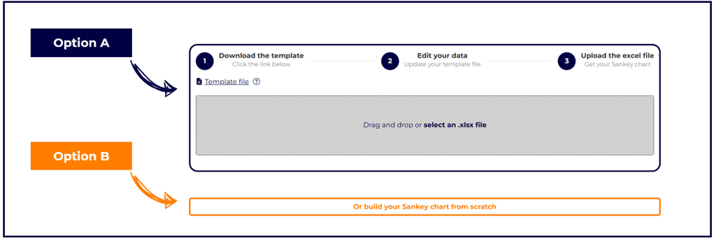
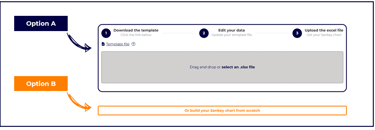
2 options (A & B) are available to build Sankey charts. For the sake of speed and convenience, we recommend using Option A.
Take a few minutes to read the instructions below and become familiar with how Sankey charts work! We promise, it is easy.
Option A
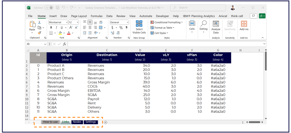
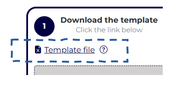
First, download our Sankey Solutions template (xlsx file). This template is needed to communicate with our online editor.
Open the template and update it with your data. 4 tabs are included in the file:
How to use (describes how to update the excel file),
Links (indicates the flows, from origin to destination, with their corresponding value),
Nodes (specifies in which order, from left to right, the nodes will appear),
Settings (allows to customize the font, decimals, prefix, suffix, and a few other things).
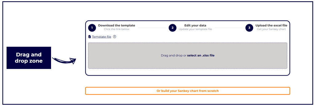
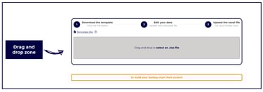
Once the excel template is updated, use the drag and drop zone.
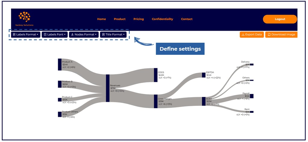
You can then access your Sankey chart in the online editor:
Proceed with font and format adjustments if needed,
Manually adjust the location of the links and nodes,
Download your image.
Option B
Alternatively, you can also build your Sankey chart directly in the online editor, without using the excel template.
In this case, the same steps as per Option A will be accomplished.


Detailed instructions (Option A)
Let's review in detail how to update each tab (Links, Nodes, Settings) in the excel template.
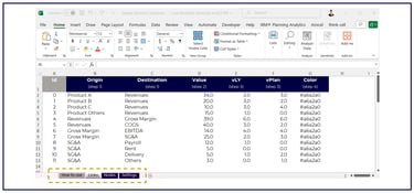
Links
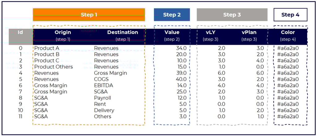
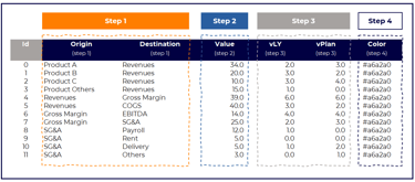
In the tab Links, 4 steps must be completed.
Step 1 (mandatory)
Define the origins and destinations of the data (e.g., from Product A to Revenues, from Revenues to Gross Margin, etc.).
Ensure each data link as an ID number.
Recommendation
Ensure that a text appearing both in Origin and Destination has the same spelling in both columns.
For example, writing "Revenues" in one column and "Revenue" in the other column would generate an error.
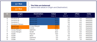
Step 2 (mandatory)
Indicate the numerical value associated with each link (for example, Product A generated $34.0M of revenues).
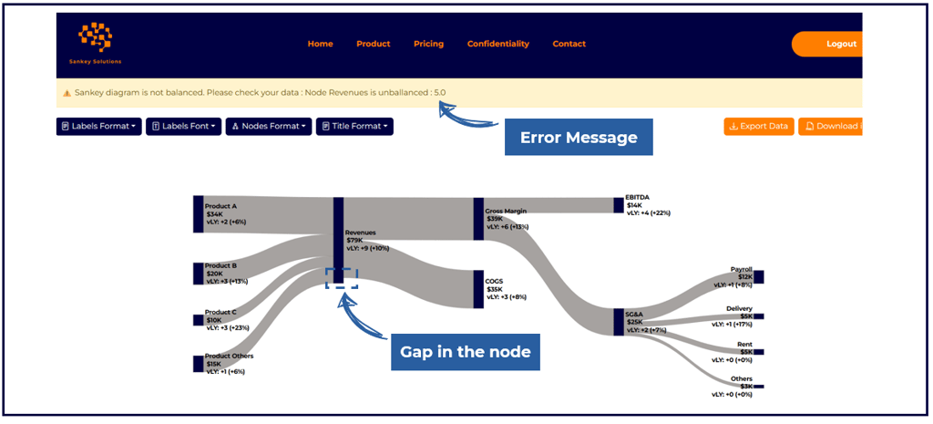
Check that the links are balanced.
When a same text appears both in Origin and in Destination, the sums must match.
For example, the 4 values for Revenues in Destination are identical in sum to the 2 values for Revenues in Origin.
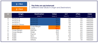
If the links are unbalanced (for example, if the flow Revenues to COGS were to indicate 35.0 instead of 40.0, so that the 2 values for Revenues in Origin would amount in sum to 74.0 instead of 79.0):
An error message would appear,
There would be a gap in the node.
Step 3 (facultative)
To include a variation (vPY and/or vPlan), indicate here the corresponding values (for example, Revenues from Product A amount to 34.0 in current year, which is +2.0 vPY year and +3.0 vPlan).
Recommendation: in the tab Settings, you can customize the wording the chart will show:
For vLY (e.g., YoY, Y/Y, vs. LY, vs. PY, etc.),
For vPlan (e.g., vFCST, vs. Budget, etc.).
Step 4 (mandatory)
Indicate the color of each flow.
Good to know: once you have updated the excel template into the online editor, you can adjust the colors again.
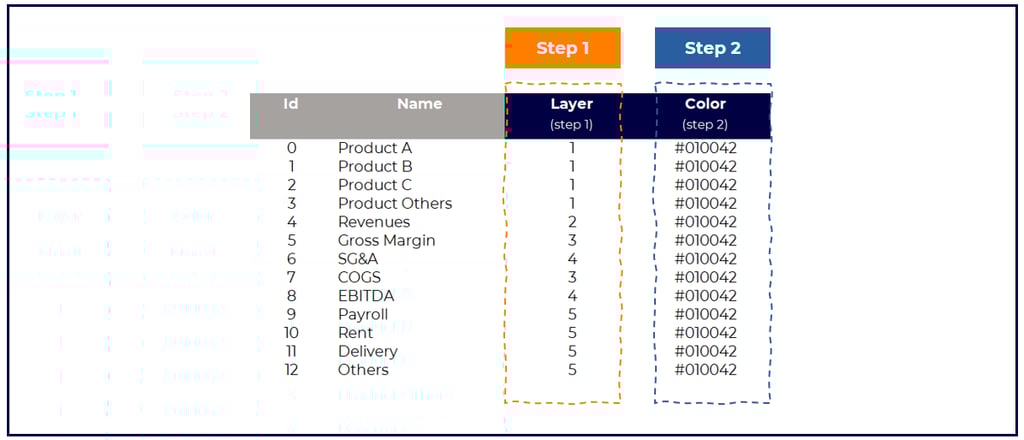
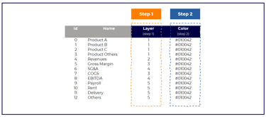
Nodes
In the tab Nodes, 2 steps must be completed.
Step 1 (mandatory)
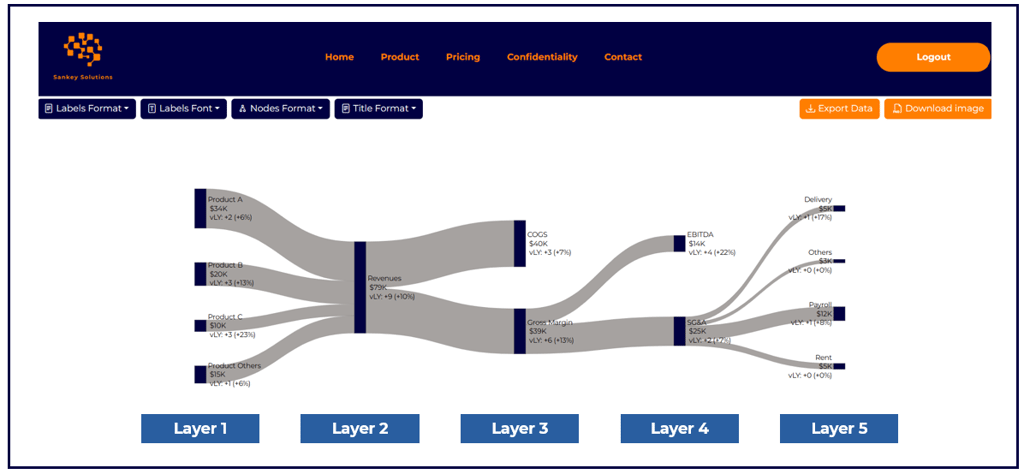
Define the layer for each node (e.g., layer 1 for all Products, layer 2 for Revenues, layer 3 for Gross Margin and COGS, etc.).
The layer indicates the horizontal order of appearance of each node, from left to right (see example below).
Step 2 (mandatory)
Indicate the color of each flow.
Good to know: once you have updated the excel template into the online editor, you can adjust again the colors.
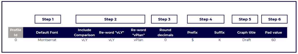
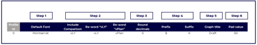
Settings
In the tab Settings, various steps can be completed for your convenience.
This tab allows you to easily determine the formatting of your Sankey chart (text font, decimals, prefix and suffix, etc.).
Step 1 - select the font of your text.
Step 2 - determine if you want your Sankey chart to include a comparison (vLY, vPlan, none) and what wording you prefer.
Step 3 - define how many decimals your Sankey chart will show (0, 1, 2).
Step 4 - select the prefix (e.g., a currency symbol such as $) and the suffix (e.g., K, M, B).
Step 5 - if you wish your Sankey chart to have a title, type here the name.
Step 6 - select the space between nodes you wish to have.
Closer to 0: the less space you will have and the thicker the links will be.
Closer to 120: the more space you will have and the thinner the links will be.
While these settings can be defined in the excel template, you can also adjust these later in the online editor.